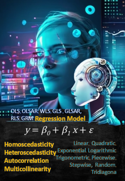
Regression Model: Overview

Welcome to Regression Model Go to User Guide

The Regression Model is a comprehensive application tool designed to offer a wide array of functionalities for estimating and fitting regression models using various statistical approaches. With intuitive options for model specification, data input, and output visualization, this tool enables users to run regression analyses anytime, anywhere.

Introduction

The Regression Model offers seamless online accessibility, allowing users to specify regression models through an interactive interface. Models are configured via a menu-driven approach, with options, buttons, and easy data import from Excel, CSV or JSON files. This user-friendly design makes fitting regression models efficient and accessible to all users.

Regression Menu

Menu Options: Fit | Output | O-Script | I-Script

1. Fit Menu:

   • Import Data File: A button to import data directly from Excel, CSV, JSON file Format, generating a data table for defining dependent (endog) and independent (exog) variables.

   • Dropdown Menu:

     • Select Regression Model:

       • OLS (Ordinary Least Squares)
       • OLSAR (Autoregressive)
       • WLS (Weighted Least Squares)
       • GLS (Generalized Least Squares)
       • GLSAR (Autoregressive)
       • RLS (Recursive Least Squares)
       • GRM (Generalized Regression Model)

     • Calculation Options:

       • Model with Intercept
       • Model without Intercept
       • Stepwise Forward Selection:
         • Statistical Prioritization
         • Explanatory Power
         • Model Simplicity

     • Sigma Generation for GLS (Generalized Least Squares):

       • Homoscedasticity (Constant Variance): Sigma = (σ² * Identity(n))
       • Heteroscedasticity (Non-Constant Variance): Linear, Quadratic, Exponential, Logarithmic, Trigonometric, Piecewise, Stepwise, Random, Tridiagonal.
       • Autocorrelation (Correlated Errors): Linear, Quadratic, Exponential, Logarithmic, Trigonometric, Piecewise, Stepwise, Random.

   • Output Options (Checkbox): Choose output details such as coefficients, VIF, covariance matrix, correlation matrix, residuals, predicted values (yHat), Sigma, weighted endog, and weighted exog.

   • Input Form:

     • Set optimization parameters for slope, rho, and base variance when generating Sigma for GLS whitening. Parameters include:
       • AR Order, Rho, Slope, Period, Step, Threshold, Base Variance, and Variance.
     • Define GRM (Generalized Regression Model) with custom functions (e.g., @b0*X0 + @b1*sin(X1) + @b2*power(X2)) and initialize parameters (e.g., {0, 0, 0} or {0.01, 0.4, 1.0}).
     • Math Functions: acos(X), acosh(X), asin(X), asinh(X), atan(X), atan2(Y,X), atanh(X), ceil(X), ceiling(X), cos(X) , cosh(X), degrees(X), exp(X), floor(X), ln(X), log(B,X), log(X), log10(X), log2(X), mod(X,Y) , pi(), power(X,Y), radians(X), sin(X), sinh(X), sqrt(X), tan(X), tanh(X), trunc(X)
     • Set Threshold Values to guide predictor selection (leave blank if no threshold is required):
       • Statistical Significance: t-Test (p-value ≤ 0.05)
       • Overall Significance: F-Statistic (Significance F ≤ 0.05)
       • Explanatory Power: Adjusted R² ≥ [...]
       • Model Simplicity: AIC ≤ [...], BIC ≤ [...]
       • Autocorrelation: Durbin-Watson (|DW - 2| ≤ 1.5)
       • Normality Tests: Omnibus Test, Jarque-Bera Test
       • Multicollinearity: Center VIF < 10
       • Heteroscedasticity: Breusch-Pagan Test (p-value > [...])

   • RUN Button: Click to compute the regression model based on selected parameters. Each run automatically stores the parameter script in the I-Script tab.

2. Output: After running the model, the results are saved in the O-Script tab, with the output report displayed in the Output tab.

   • Regression Output:

     • Model equation: Y = f(X)
     • Stepwise Regression (Forward Selection) for Stepwise Case :
     • Decision criteria: Statistical prioritization with thresholds for p-value, F-statistic, Durbin-Watson statistic, VIF, and more.
     • Predictor Analysis: P(t), F-Statistic, Adjusted R², AIC, BIC, Intercept, Slope.
     • Additional Statistics: Includes predictors, significance tests, variance inflation factors (VIF), and diagnostics for residuals.
     • Regression Statistics:
     • Multiple R, R², Adjusted R², Standard Error, Durbin-Watson statistic, and ANOVA output.
     • Coefficients for each predictor along with standard errors, t-statistics, and p-values.
     • Diagnostic Statistics:
     • Omnibus test, Jarque-Bera test, Durbin-Watson, Log-Likelihood, AIC, BIC, Breusch-Pagan test, and their associated p-values are all computed to assess model fit and reliability.

3. O-Script and I-Script: After running the model, the results are saved in the O-Script and I-Script tab.

   • O-Script: Allows editing of the output script to customize the report generation.
   • I-Script: Provides input script editing for modifying model settings and parameters prior to running the regression analysis. This also provides able to tranform data suporting both Math and Aggregate Funtions to generate data table
   • Math Funtions: acos(X), acosh(X), asin(X), asinh(X), atan(X), atan2(Y,X), atanh(X), ceil(X), ceiling(X), cos(X) , cosh(X), degrees(X), exp(X), floor(X), ln(X), log(B,X), log(X), log10(X), log2(X), mod(X,Y) , pi(), pow(X,Y), power(X,Y), radians(X), sin(X), sinh(X), sqrt(X), tan(X), tanh(X), trunc(X)
   • Aggregate Functions: min(expr), max(expr), count(), sum(expr), avg(expr)